
There are many ways of achieving similar results when it comes do analyzing and working with data. I am a big fan of flexibility and taking advantage of what each method has to offer.
Some options will be better for working with larger databases while other will do a good job with small ones. Some might be suited for those who are not so well versed with a programming language like Python and others will offer a wider range of resources for dealing with any situation.
As someone with quite some experience on working with spreadsheets, naturally they become an easy go-to way to start analyzing data. However, the two-dimensional way of representing information on the screen will likely become a barrier, even with all lookups and pivot tables in the world. That is why learning a proper database language like SQL is very handy.
While SQL can get quite complex when tables and relationships become numerous, it is also useful even for simple tasks, specially because its syntax is not so scary, being even similar to plain english.
This will be the first post of a series where I will discuss some ways of integrating SQL and SQL-like commands to databases and spreadsheets.
Google Sheets and the QUERY function
Google Sheets is great. It saves automatically on the cloud, so it can be accessed anywhere and is amazing to share and colaborate. There is a perfect integration with Forms and an interesting integration with other apps like Docs, Slides and Sites to create nice presentations.
I particularly use Sheets more often than Excel. I have a Chrome Browser dedicated to open .xls files, with a plugin to open them directly with Google Drive apps. I like the clean interface and I am used to the functions, syntax and charts. This came from necessity of sharing the spreadsheets and working on them real time, and now I find it great.
It has some limitations, specially when data starts to get bigger. I have tried to work with hundreds of thousands of lines and it was not good, to say the least. But that is not really the goal of this tool. This is for a day-to-day simple use, with some sophisticated tools to make it more interesting.
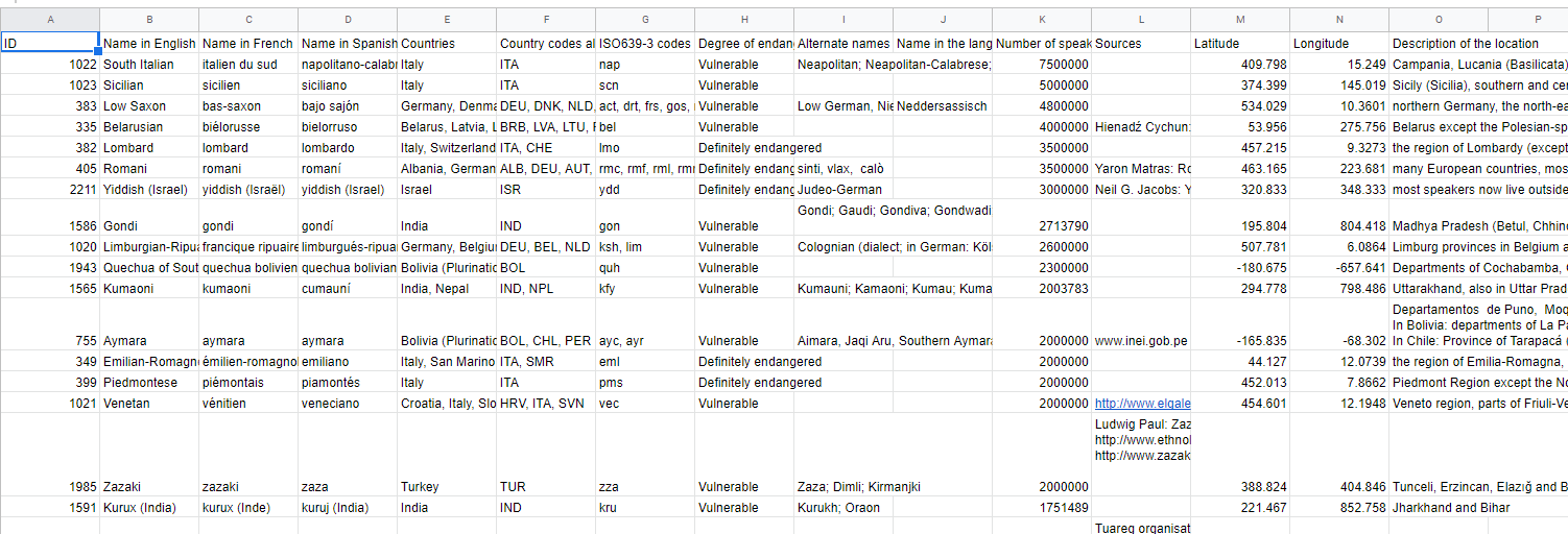
I will work with a dataset downloaded from Kaggle, uploaded by the newspaper The Guardian, that contains information about extinct and endangered languages throughout the world. The link for the dataset is here.
Importing and getting data ready
With Google Sheets, importing .csv data is very easy. Just File > Import and then select the file. Depending on what you select it will open a new spreadsheet, file, or replace the current open one. The initial data looks like this then:
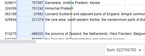
If the original file was in a good format we can continue right away, but if we need to clean up a little bit, we can also do it. A good way to start is to apply filters to all the columns to make it possible to select some values and see if it works fine. A nice trick can be done on columns that are expected to receive numbers: select the entire column of interest and check if you can see the sum of the values. If you can’t, probably there are some strings in the middle. The solution is to just select the column, click Format > Number > Automatic, or any other format needed.
When we decide to start working with our queries, a good practice is to create a new spreadsheet inside the file.
Because the function QUERY will not use the column headers, but the letters of the spreadsheet, it can be useful to have a small cheat-code with the column names so we can know what we are selecting. This is definitely not mandatory though.
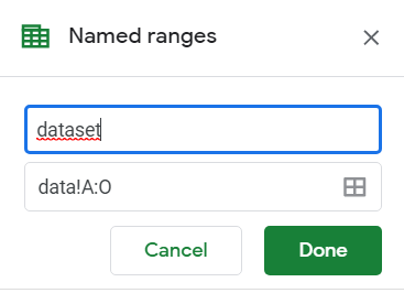
In the data sheet we can select all the columns we have information on and then click Data > Named ranges. We will see a box like this to create a name for this range to be used in future references:
Creating a Query
Now, on the new spreadsheet we will use on the A1 cell the function QUERY. The function has three parameters: which table will be searched; the SQL-like command; and if the table has or not headers.
When we start typing the table name we see this:
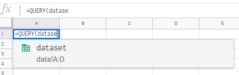
An autocomplete feature is good when we have more named ranges, so we can select the correct one while writing the function.
A big difference from SQL is that here we specify the table for the function and then the select command afterwards is related to that table, so we don’t use the traditional select * from table. If we want to show the entire data, we type:
=QUERY(dataset;"select *")
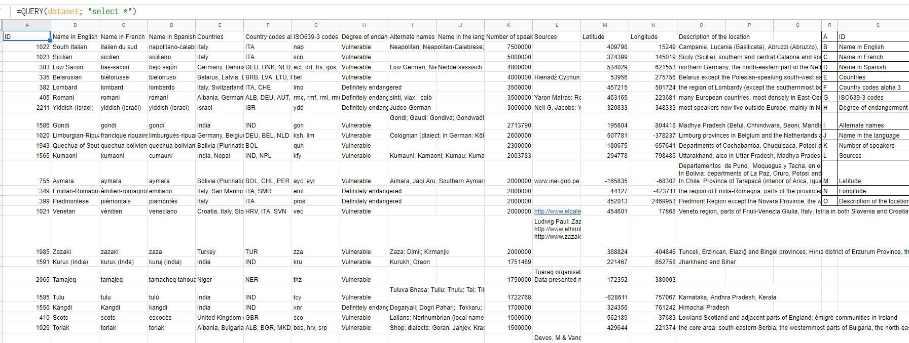
Using the function on the A1 cell will make the query show its results on all the next columns and rows that are empty. It is important then to have “clear space” on the spreadsheet. Selecting any cell other than the A1 will show the data as a value, not as a formula.
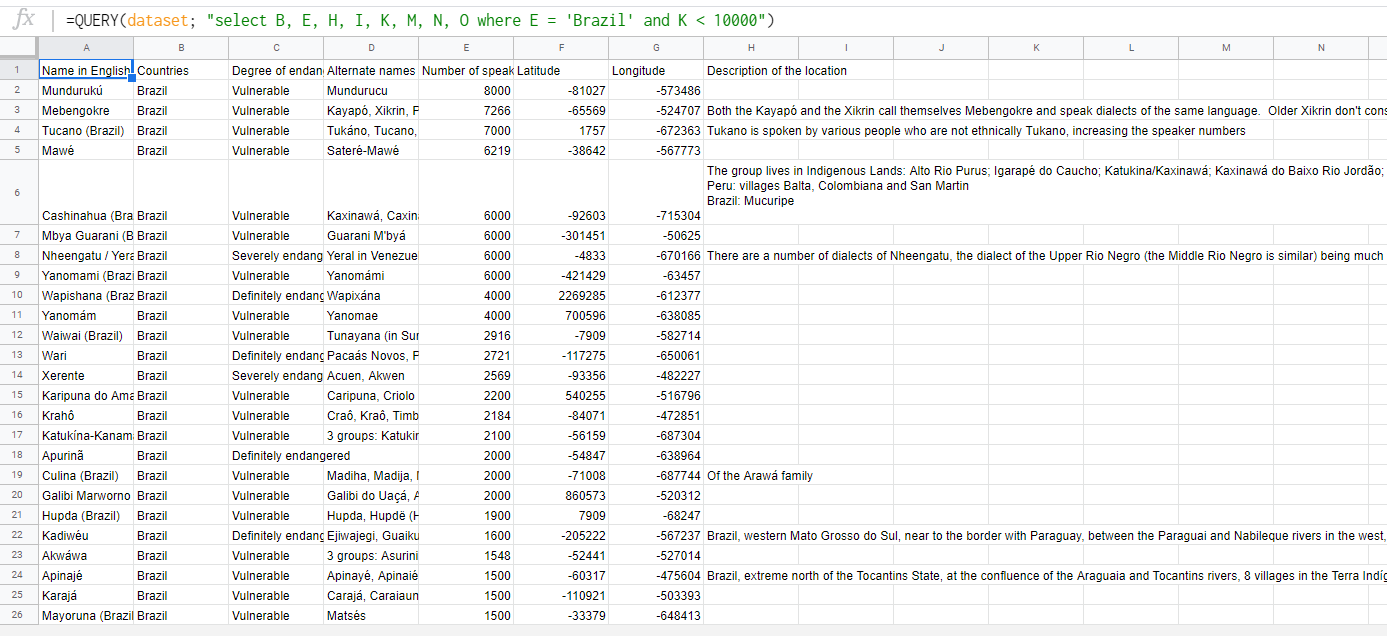
We can now make filters, ranks and aggregations for example.
=QUERY(dataset;"select B, E, H, I, K, M, N, O where E = 'Brazil' and K < 10000")
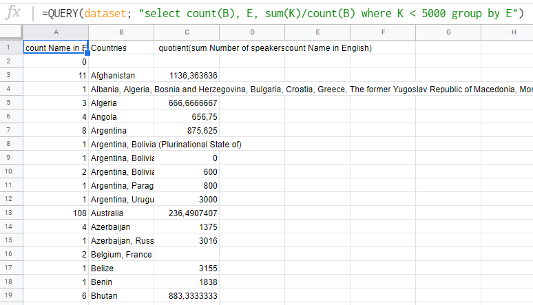
=QUERY(dataset;"select count(B), E, sum(K)/count(B) where K < 5000 group by E")
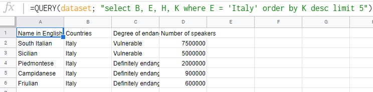
=QUERY(dataset;"select B, E, H, K, where E = 'Italy' order by K desc limit 5")
This already is a very powerful way to filter data. Google Query Language documentation has the entire list of commands to be used.
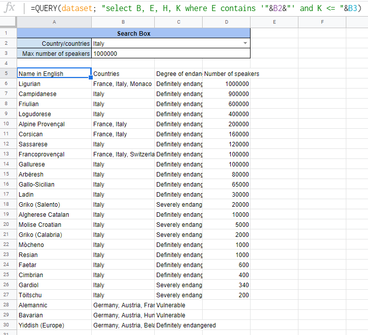
We can make things easier for users that are not so experienced with spreadsheets and create an interactive query tool as well. While this will require some work in order to be sure to give plenty of flexibility to the user for the data search, a simple demonstration could be like this:
=QUERY(dataset;"select B, E, H, K where E contains '"&B2&"' and K <= "&B3)
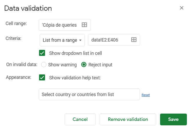
The dropdown menu can be done with a right click on the cell and then selecting ‘Data Validation’.
We can also have some automated charts. In this example I show a simple example where we plot a bar chart with the top-10 languages in terms of number of speakers (when they have equal or less than 1 million people speaking them).
The title of the chart is written on a normal cell, with some concatenation to get the name of what was written in the Country/Countries field.
Another interesting tip is that the query can perfectly be hidden in another spreadsheet (or maybe just put the chart on top of the query result) and the final user can have access only to the search box and the chart.
It is important that the chart should not be limited by its own parameters; that means that the user shouldn’t put the number of rows to be plotted. Rather than that, the best idea is to just select the entire columns (or, in this case, A6:D) and use the limit command to specify how many observations will be selected.
Conclusion
Google Sheets is a great free tool that allows some very nice creations using not so big datasets. There are some issues, mainly the lack of a join command to join and merge different tables. It can still be done, however it is not optimal. We will explore these options on future posts.
For simple work and for dealing with online Google Forms, this kind of approach using QUERY, automated charts and other kind of reports is amazing and produces good and quick results.